Identifying various types of insects can be advantageous for humans. For example, recognizing specific butterflies can enhance plant reproduction, while identifying other insects can determine if they are dangerous, aiding veterinarians in making initial diagnoses. By knowing this, you will be able to see how they live and interact with specific types of insects. For instance, you do not want to hurt insects that can eat pests in your garden, and many more examples that you can get by identifying types of insects. Yet, one question comes to mind,
Have you ever thought to classify insects using technology? Is it possible to do?
Absolutely, It is really possible to do. You are going to classify types of mosquitoes on human skin by using TensorFlow.
By carrying out a deep learning model based on the data available, you can identify each type of insect and determine the species composition of mosquito fauna at a given place and time for longer research. This is essential for the research or something useful for future purposes whether it is new knowledge for the textbook to consume or for someone who is going to research it as a reference. Moreover, you can understand the type of pest for a specific type of mosquito. Before delving deeper into this experimentation, I recommend reading part 1 of 2 where I explained fundamental things about solving image data problems using Tensorflow and what you need to know to successfully implement it.
In this experimentation, you will classify the type of mosquito on human skin on the multiclassification problem. There are 6 classes of mosquito namely albopictus landing, albopictus smashed, aegypty landing, aegypty smashed, culex landing, and culex smashed as shown in the following images.
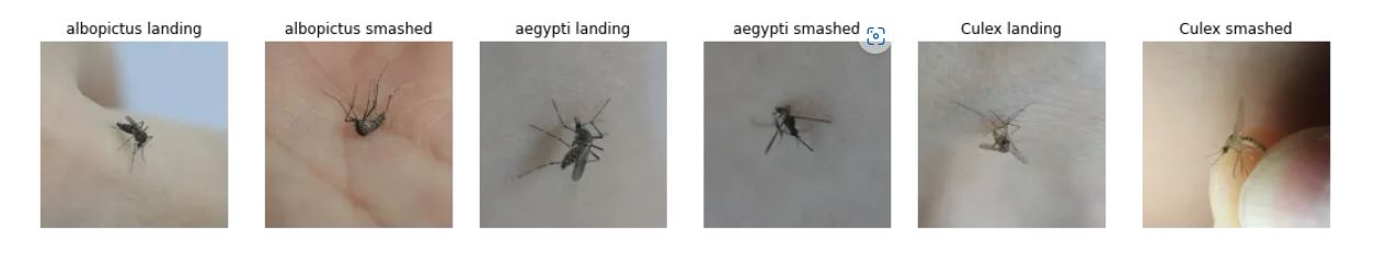 6 classes of mosquito types
# Dataset split
train_dir = "/content/zw4p9kj6nt-2/data_splitting/Train/"
valid_dir ="/content/zw4p9kj6nt-2/data_splitting/Pred/"
test_dir = "/content/zw4p9kj6nt-2/data_splitting/Test/"
# Create data inputs
IMG_SIZE = (224, 224) # define image size
train_data = tf.keras.preprocessing.image_dataset_from_directory(directory=train_dir,
                                                                            image_size=IMG_SIZE,
                                                                            label_mode="categorical", # what type are the labels?
                                                                            batch_size=32) # batch_size is 32 by default, this is generally a good number
val_data = tf.keras.preprocessing.image_dataset_from_directory(directory=valid_dir,
                                                                           image_size=IMG_SIZE,
                                                                           label_mode="categorical")
test_data = tf.keras.preprocessing.image_dataset_from_directory(directory=test_dir,
                                                                           image_size=IMG_SIZE,
                                                                           label_mode="categorical",shuffle=False)
Preprocess Images
The Mosquito on human skin is a dataset provided by researcher Song-Quan Ong who wanted to contribute more to classifying the type of mosquito on human skin. You can check further details on the link given. The dataset has been already split into 3 parts training(Train), validation(Predict), and Test data. Each split has balanced 6 classes of mosquito types.
You can check the code above where we preprocess the images into their proper size 224 *224 with 3 color channels. We use tf.keras.preprocessing to preprocess them. Again you can check part 1 of this article where I explained a handful of ways to preprocess images. One of them is tf.keras.preprocessing. The advantage of using it is the usage of handling data faster and a few features like carrying out training optimization, batching, and optimization of tensor computation that are beyond the scope of this article. You can also use another class provided by Tensorflow like the ImageGenerator instance. I prefer using tf.keras.preprocessing for this article.
The code above explained how we preprocess the images based on a dataset split into training, validation, and test data with a similar size. We also use batch size 32 to help gradient descent converge faster when doing backpropagation during training on deep learning models. I also explained why batch size is essential when training deep learning models when they fitted into the images/data in the previous article.
Your Tensorflow Pocket References on Image Data Task How can you build Deep Learning Models using Tensorflow for Image Data Task? medium.com
Modeling and Making Inference
# 1. Create base model with tf.keras.applications
base_model = tf.keras.applications.EfficientNetB0(include_top=False)

# 2. Freeze the base model (so the pre-learned patterns remain)
base_model.trainable = False

# 3. Create inputs into the base model
inputs = tf.keras.layers.Input(shape=(224, 224, 3), name="input_layer")

# 4. If using ResNet50V2, add this to speed up convergence, remove for EfficientNet
# x = tf.keras.layers.experimental.preprocessing.Rescaling(1./255)(inputs)

# 5. Pass the inputs to the base_model (note: using tf.keras.applications, EfficientNet inputs don't have to be normalized)
x = base_model(inputs)
# Check data shape after passing it to base_model
print(f"Shape after base_model: {x.shape}")

# 6. Average pool the outputs of the base model (aggregate all the most important information, reduce number of computations)
x = tf.keras.layers.GlobalAveragePooling2D(name="global_average_pooling_layer")(x)
print(f"After GlobalAveragePooling2D(): {x.shape}")

# 7. Create the output activation layer
outputs = tf.keras.layers.Dense(6, activation="softmax", name="output_layer")(x)

# 8. Combine the inputs with the outputs into a model
model_2 = tf.keras.Model(inputs, outputs)

# 9. Compile the model
model_2.compile(loss='categorical_crossentropy',
              optimizer=tf.keras.optimizers.Adam(),
              metrics=["accuracy"])

# 10. Fit the model (we use less steps for validation so it's faster)
history_2 = model_2.fit(train_data,
                        epochs=10,
                        steps_per_epoch=len(train_data),
                        validation_data=val_data,
                        # Track model training logs
                        callbacks=[create_tensorboard_callback("CNN_learning", "transfer_learning_efficientNet_0")])
I tried a lot of experiments on this dataset from carrying out CNN from scratch using TensorFlow, tuning hyperparameters, trying out various transfer learning models, and finding EffiecientNetB0 with hyperparameter tuning has been giving a better accuracy(~90%) as shown on the code above. I use tf.keras.application to download EfficientNetB0 to be used for training our specific dataset in this case our mosquito on human skin. You can see how easy to implement transfer learning using Tensorflow. You can see the model architecture of EfficientNetB0 which is developed by Google in the paper for more details. Based on my experiences competing in the Kaggle competition, I often see people use EfficientNet as a Backbone/baseline for computer vision competition. It is like XGBoost for tabular data competition if you are quite familiar with the competition in Kaggle. In the following EfficientNetB0 model architecture where we have input data of its size 224*224(we preprocess and suit our data). Again, because transfer learning model architecture is beyond the scope of making this article, I consider reading the paper is a better way to understand the model architecture as shown in the following
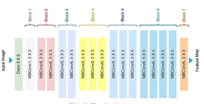
EfficientNetB0 model architecture You can see with just a handful of lines of code you can implement EfficientNetB0 with data that has been preprocessed based on the model architectures. One essential takeaway is that we add one hidden layer for getting output using the softmax activation function to get the predicted probability of the images. The largest predicted probability will be the prediction based on the 6 classes of mosquito type on each image tested on our trained model. You can see it on my Kaggle notebook
where I tried out various preprocessing data like data augmentation and transfer learning model architecture or CNN from scratch using Tensorflow. You will see how transfer learning with hyperparameter tuning outperforms the CNN model carried out from scratch. CNN model just gave around 70% compared to 90% of using transfer learning. One important thing to note is to use all the outputs based on the data used on the transfer learning model architecture or suit based on our specific task. In this case, you are going to choose 6 classes as output rather than using all outputs on EfficientNetB0. We do this by changing the parameter include_top=False when making the base_model instance and changing the output into 6 classes and using the softmax activation function. Then, we compile the model and choose the loss function and Adam Optimization for helping gradient descent converge faster. In many implementations of deep learning models when fitting into the data, most deep learning practitioners often use Adam Optimization because it can change the learning rate to converge to reach a global minimum. After fitting the data and finishing the training process, you can plot for comparing the loss and accuracy of train and validation data. It is shown in the following plots where the loss decrease as the epochs reach 10 epochs and the accuracy increase as the epochs reach 10 epochs to around 90%.
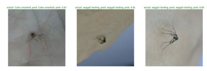
The Comparison of Loss and Accuracy on training(TRAIN) and validation data(PRED) You can visualize how effective our trained model is by comparing the ground truth and predicted classes as shown in the images below. You can see from these 3 test images, we predicted them correctly with predicted probability shown as an annotation in understanding it better.
# Make preds on a series of random images
import os
import random

plt.figure(figsize=(20, 14))
for i in range(3):
  # Choose a random image from a random class
    class_name = random.choice(class_names)
    filename = random.choice(os.listdir(test_dir + "/" + class_name))
    filepath = test_dir + class_name + "/" + filename

    # Load the image and make predictions
    img = load_and_prep_images(filepath, scale=False) # don't scale images for EfficientNet predictions
    pred_prob = model_3.predict(tf.expand_dims(img, axis=0)) # model accepts tensors of shape [None, 224, 224, 3]
    pred_class = class_names[pred_prob.argmax()] # find the predicted class

    # Plot the image(s)
    plt.subplot(1, 3, i+1)
    plt.imshow(img/255.)
    if class_name == pred_class: # Change the color of text based on whether prediction is right or wrong
        title_color = "g"
    else:
        title_color = "r"
    plt.title(f"actual: {class_name}, pred: {pred_class}, prob: {pred_prob.max():.2f}", c=title_color)
    plt.axis(False);
Code for comparing test images and ground truth labels
 The comparison between Ground truth and prediction classes
You can see on the first image of our comparison between ground truth and predicted classes where the ground truth is culex smashed and our predicted class is also culex smashed. It is similar to aegypty landing as ground truth and predicted classes on the second image and third one.
The comparison between Ground truth and prediction classes
You can see on the first image of our comparison between ground truth and predicted classes where the ground truth is culex smashed and our predicted class is also culex smashed. It is similar to aegypty landing as ground truth and predicted classes on the second image and third one.
Evaluation
Evaluation plays an important part after the modeling process finishes. Even though in real life as machine learning practitioners, we will do a Machine learning loop process where we will always evaluate again and again to see the performance of our trained model that tends to degrade over time. Then, you need to evaluate the trained model in the new images(Test data) to see how effective our trained model is tested on unseen data based on patterns we get from training the TRAIN data. Because we do an image classification problem, many people use the accuracy score to see how effective our model is when the data is balanced. The accuracy score is the fraction of the predictions our model got right. Our dataset is quite balanced for each split in the Train, predict, and test data. We can use accuracy for this case. We can use the scikit-learn library to get accuracy_score like the code as follows
# Get accuracy score by comparing predicted classes to ground truth labels
from sklearn.metrics import accuracy_score
sklearn_accuracy = accuracy_score(y_labels, pred_classes)
sklearn_accuracy
Accuracy Score implementation on Scikit-learn With this code, we compare our ground truth or y_labels with the prediction (the largest predicted probability in test data ). The higher the score, the better accuracy we get. In this experiment after tuning a handful of hyperparameters like learning rate, how many epochs to run, and trying out Early Stoping, we get around a 90% accuracy score. You can check the code in the notebook.
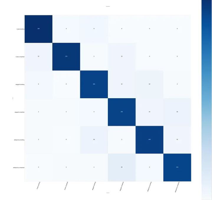
In addition to that, you can see the visualization of how effective our accuracy score is by visualizing the predicted label and the ground truth on the confusion matrix table in the following images
Confusion matrix for multiclass classification
 Confusion Matrix
The X-axis shows the predicted labels and the y-axis shows the ground truth. The darker the diagonal part of this table, the better score we get as shown in the image above where we get fewer labels misclassified from our 90 % accuracy score. You can also see how we code the confusion matrix on the notebook for further details.
TensorBoard Dev
Tracking our machine learning model is a good way to monitor the performance of our model. You can see on the image as follows where we track our accuracy score on various deep learning models and upload it to tensorboarddev. This is one of the advantages of using Tensorflow where we can track our trained model and share it publicly. You can check the first part of 2 parts where I explained tensorboard and how to upload your evaluation metrics score to tensordboard.dev. you can track the graph by visiting this tensorboard.dev
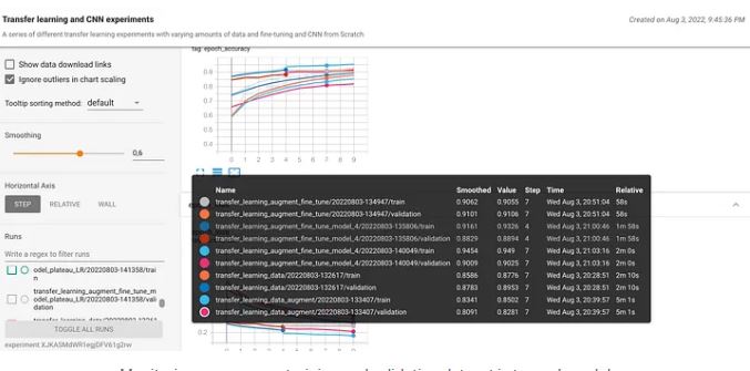 Monitoring accuracy on training and validation dataset in tensorboard dev
Conclusion
Image Classification is the most used in many sectors for identifying the taxonomy of animals, medical imaging, logistics, automotive, etc. It is used in many use cases where we identify particular images and predict the labels of particular images. You can see in our experiments where we predict the type of mosquito using Tensorflow. Having a piece of good knowledge of classifying images is a good thing for deep learning practitioners for making an impact on society.
References
Ong, Song-Quan (2022), “Mosquito-on-human-skin”, Mendeley Data, V2, doi: 10.17632/zw4p9kj6nt.2 on Mosquito-on-human-skin dataset
Thank you for reading! I really appreciate it! 🤗 If you liked the post and would like to see more, consider following me. I post topics related to machine learning and deep learning. I try to keep my posts simple but precise, always providing visualization, and simulations.