Developing machine learning applications require numerous steps. Gathering the data, doing data cleaning, exploring the data through exploratory data analysis, feature engineering, feature selection, modeling, evaluation, and interpretation. Interpretation is one of the crucial parts of developing a machine learning application. This process requires a lot of scrutiny due to the business requirement. Machine learning engineers require to set out how the machine learning model makes a certain prediction on the data to the nontechnical businesspeople/stakeholders.
Imagine if you are using a neural network model with complex features for developing your machine learning application, Will the nontechnical businesspeople trust your model prediction? Absolutely no. It is likely to be a big problem for the stakeholders to speed up the business processes using machine learning due to the intricacy of the models. Thus, the ability to interpret the model is essential knowledge to know for making nontechnical businesspeople to trust our machine learning model when making a specific prediction on the data.
Shap (Shapley Additive exPlanations) is one of the most of Explainable Artificial Intelligence(XAI) tools to interpret why machine learning models make a specific prediction on the data instances. Shapley Additive exPlanations employs shap value in order to explain the prediction made by machine learning model. Shap value is based on the game theory approach to making a prediction.
Imagine you are participating in a machine learning hackathon with your team that consists of 4 members. Everyone has their own unique abilities in order to approach the problem given in the hackathon. If your team won the hackathon, how would you decide on the fair payout for the particular member of the contribution given by a particular member.
It is definitely wise to break down a distinct portion of the payout for a particular member. That is the same with how shap interpret our model based on the data we train on the machine learning model. Mathematically speaking, this is a complex thing to explain. You can check the research paper of the mathematical explanation for this interpretable tool and their GitHub repository for the update features.
We will walk through an example to implement shap for telco churn dataset that we can download on Telco Customer Churn Focused customer retention programs
This dataset contains 7043 customers and 21 features to predict whether the customers will churn or not based on data instances. We are not diving deeper into the complete machine learning process here. I just do a simple exploratory data analysis and preprocessing data.
It is recommended to make a proper exploratory data analysis, data cleaning, feature engineering, feature selection, cross-validation, and evaluation steps in order to get a much better prediction of the data instance. We are mainly focused on the implementation of Shap for interpreting the models for this tutorial.
You can take a look at the implementation in this notebook for your reference.
Interpreting Result
The first thing we need to do before interpreting the result is to train our machine learning model on the training data. On this dataset, we employ XGBoostClassifier for solving this classification problem to look into the customers who churn or not as shown in the following code.
model = XGBClassifier(n_estimators = 50, random_state = 42)
model.fit(x_train, y_train)
XGBClassifier(base_score=0.5, booster='gbtree', callbacks=None,
              colsample_bylevel=1, colsample_bynode=1, colsample_bytree=1,
              early_stopping_rounds=None, enable_categorical=False,
              eval_metric=None, gamma=0, gpu_id=-1, grow_policy='depthwise',
              importance_type=None, interaction_constraints='',
              learning_rate=0.300000012, max_bin=256, max_cat_to_onehot=4,
              max_delta_step=0, max_depth=6, max_leaves=0, min_child_weight=1,
              missing=nan, monotone_constraints='()', n_estimators=50, n_jobs=0,
              num_parallel_tree=1, predictor='auto', random_state=42,
              reg_alpha=0, reg_lambda=1, ...)
Shap works as a surrogate model to interpret our machine learning model prediction using shap value. We have to get this value using the following code. We instantiate the shap object and test the shap algorithm to our test data.
explainer = shap.Explainer(model)
shap_values = explainer(x_test)
Shap framework has the ability to interpret the data based on 2 approaches namely local Interpretability and global Interpretability. Local interpretability is the way how shap interprets the data based on a specific data instance whereas global interpretability interprets the data on the holistic features and data we have. Oftentimes, It is better to predict based on a particular data instance over all the data due to different interpretations and results. We will be visualizing the global interpretability and local one for our own use cases.
Global interpretability with feature importance
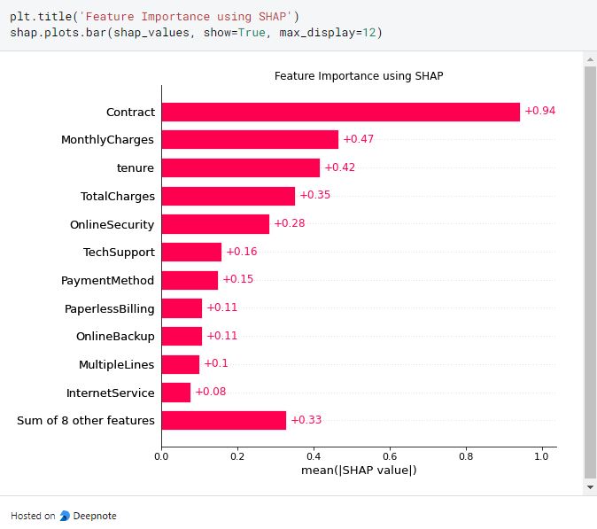
The preceding barplot shows how each feature impacts the prediction we make on training data based on the machine learning model we employ. We can see Contract feature has the most significant influence on predicting the target outcome followed by MonthlyCharges and tenure.
Global interpretability with heatmap plots
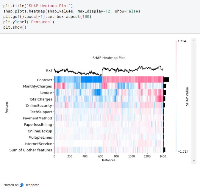
The heatmap shows the impact of all features on the model. We can see the increase contract feature will also increase tenure and TotalCharges in the red region due to the higher shap value for these features. The f(x) curve on the top shows how the predicted Churn with the increase of data instances. We can see how the Churn predictions influence the increase of the data instances.
Global interpretability with hierarchical
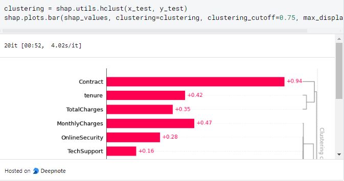
This plot shows that feature tenure and TotalCharges form a group and OnlineSecurity and Multiplines form another group. This process is then called hierarchical clustering. This graph also shows how a handful of features have some interaction based on the subgroup and it could be a feature that we can detect in our EDA for further analysis.
Global interpretability with SHAP summary plots
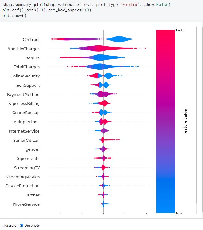
The violin plots show the positive or negative impact of the feature for some data points. TotalCharges shows a positive correlation with the target outcome because of the red color gradient. However, it differs with Contract, tenure, and TotalCharges in which low values indicate churn.
Global interpretability with feature dependence plot
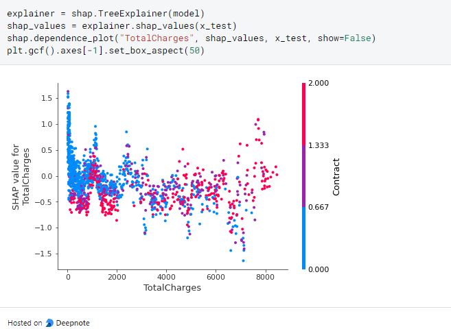
A feature independence plot is like a scatterplot where we can look at the correlation of two variables. The visualization shows the increase of TotalCharges will increase the Contract too.
Local interpretability using Waterfall plots
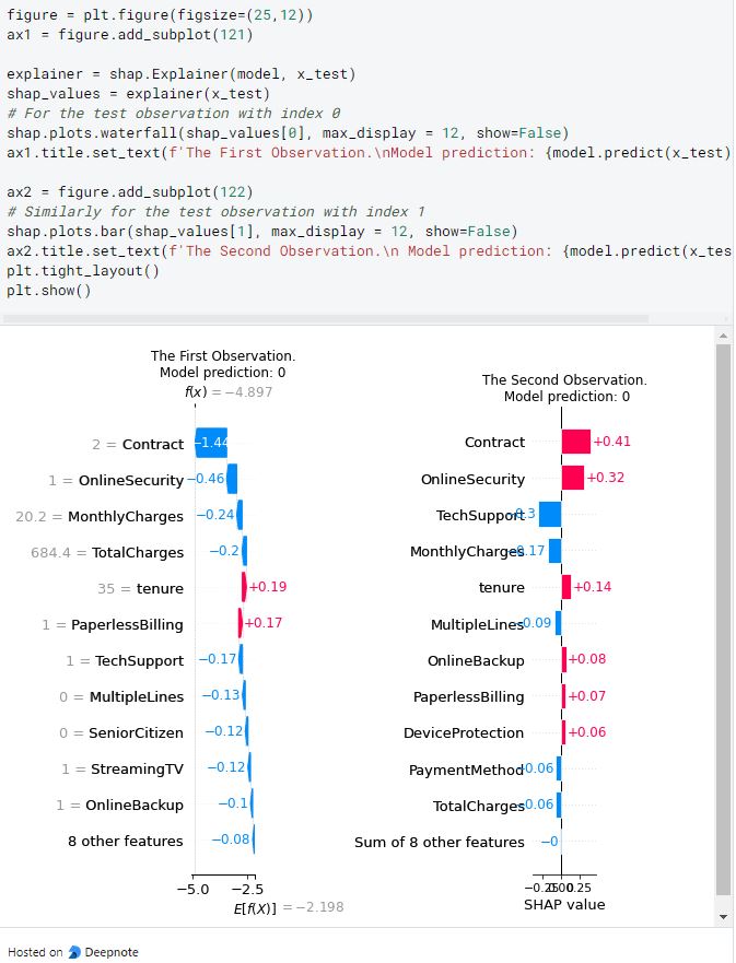
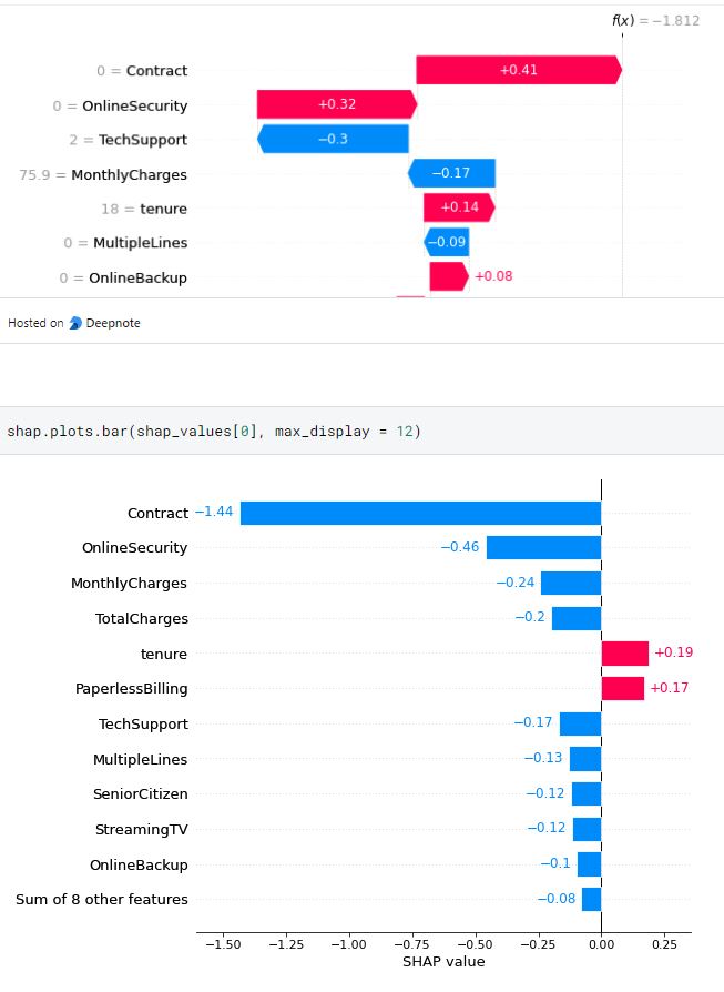
we can see from an inference of data instance towards the features on the first and second observation shows different results in which on the first observation, the contract feature contributes negatively towards the model prediction whereas the contract feature contributes positively towards the model prediction on the second one.
Local interpretability with decision plot
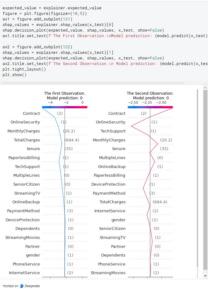
Decision plots help the interpretability to handle many features in our dataset to interpret. We can see from the preceding plots how each current local predictions are higher or lower than the average predicted outcome and how the value of the features is affecting the model outcome. In the two examples shown, the cases features contract to TechSupport are negatively impacting the model while most features on the second observation are positively impacting the model prediction.
You can also read my article related to Explainability AI (XAI) published by Freecodecamp
References:
[1]. Scott M. Lundberg. “A Unified Approach to Interpreting Model Predictions”. (2017).
[2]. Scott M. Lundberg. “Shapley Additive Explanations”. (2017).
Thank you for reading!
I really appreciate it 🤗. I post machine learning and deep learning- related topics. I try to keep my posts simple but precise, always providing visualization, and simulations.